10 Working with Qualitative Data in R
The main package we use to analyze qualitative (i.e, non-numeric) data in R is tidytext, which by the name you may have already guessed is designed to work with tidyverse packages and tidy data principles.
Before starting make sure to install.packages("tidytext"). Also, if you want to make a word cloud visualization later in this tutorial, also install the wordcloud package. Then, read in the libraries:
library(tidyverse)
library(tidytext)
library(wordcloud)
You should download the Qual Methods Survey.xlsx file from Canvas and put it in the data/ folder you’ve been using throughout class (within an R Project). Then run the following chunk of code, which uses readxl (which should already be installed with RStudio) to read in an Excel file. We also have to specify which sheet of the excel file to read in.
data <- readxl::read_excel("data/Qual Methods Survey.xlsx",
    sheet = "Form1")
Now, let’s analyze one question at a time.
10.0.1 Is Science Objective?
The first one was a short, ‘Yes’ or ‘No’ in response to the question ‘Do you think science is objective?’.
We can make a quick plot to summarize the responses:
data %>%
  ggplot(aes(x = `Do you think science is objective?`))+
  geom_bar()+
  #adds the actual count value to the chart
  geom_text(aes(label = after_stat(count)), stat = "count", vjust = 1.5, size = 12, color = "white")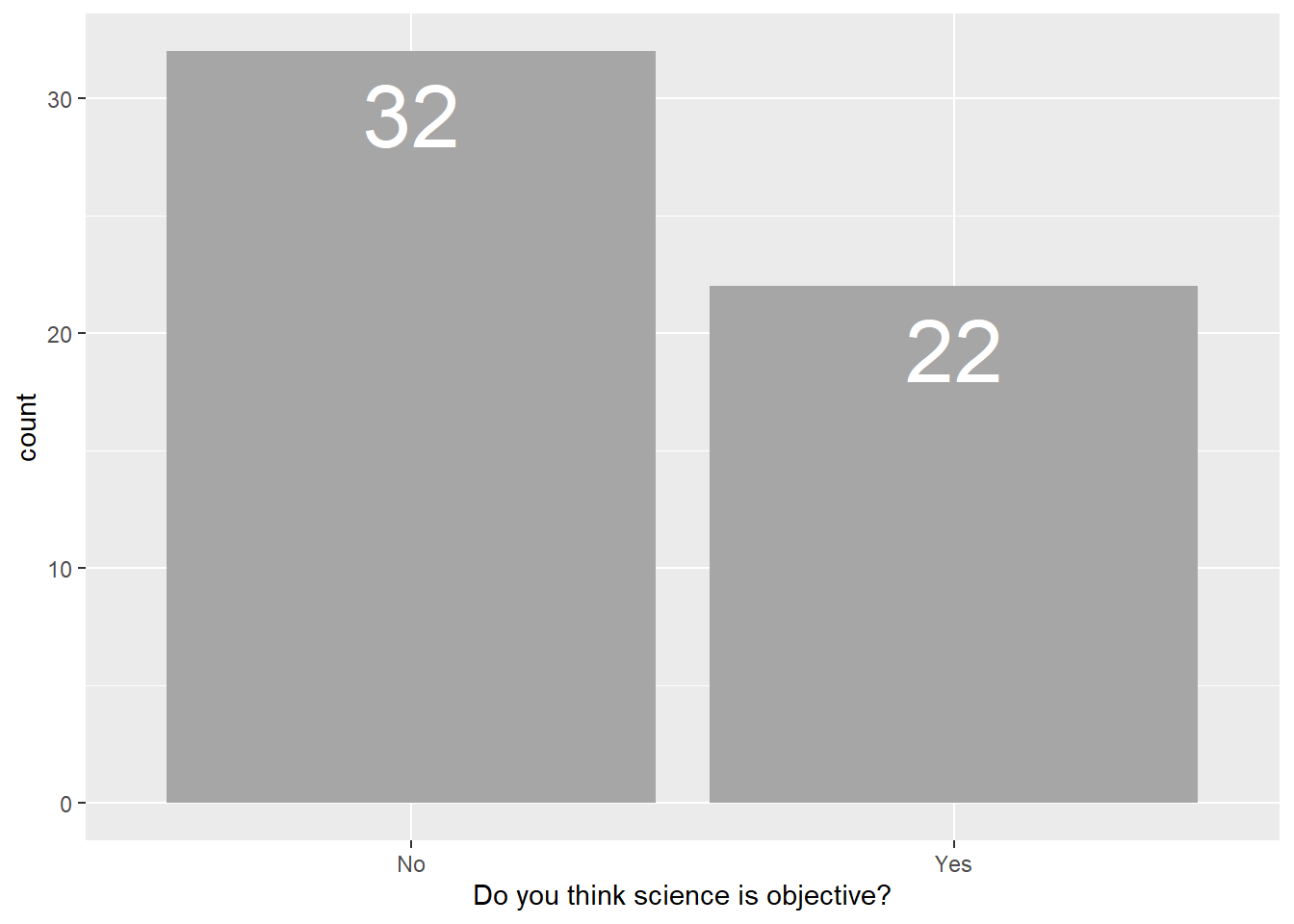
Note that since we have spaces in our column headers, we must put the title within ` ` or ” “.
Now the next question was an open ended follow up, “Why or Why Not?”
Before we conduct the text analysis, lets split our data in two, those that said ‘yes’ and those that said ‘no’.
yes <- data %>%
  filter(`Do you think science is objective?` == "Yes")


no <- data %>%
  filter(`Do you think science is objective?` == "No")
Let’s analyze the ‘Yes’ responses first.
First, we always set up the text analysis by using the tidytext function unnest_tokens() which will tokenize the text for us, meaning taking the full responses and separating each word out into its own row becoming a unique observation. You can also separate responses by consecutive words (i.e., ngrams), sentences, and more by changing the token =argument, which we will do later.
There is a second step we want to add to this process, which is to remove ‘stop words’, removing noise in the data. tidytext has a built in data frame of these stop words in English called stop_words.
stop_words## # A tibble: 1,149 × 2
## word lexicon
## <chr> <chr>
## 1 a SMART
## 2 a's SMART
## 3 able SMART
## 4 about SMART
## 5 above SMART
## 6 according SMART
## 7 accordingly SMART
## 8 across SMART
## 9 actually SMART
## 10 after SMART
## # … with 1,139 more rows
## # ℹ Use `print(n = ...)` to see more rowsWe remove these stop words from our data frame with the anti_join() function, which keeps all the words that are NOT found in stop_words. To easily anti_join(), we want to also name the new text column we create from unnest_tokens() word.
So, to prepare our data set for text analysis the code looks like this:
yes_why <- yes %>%
  #keep just our column of interest
  select(`Why or why not?`) %>%
  unnest_tokens(output = word, #the new column name to put the text in
                input = `Why or why not?`)  %>%
anti_join(stop_words, by = "word") # remove any stop wordsyes_why## # A tibble: 150 × 1
## word
## <chr>
## 1 based
## 2 evidential
## 3 reasoning
## 4 science
## 5 deals
## 6 finding
## 7 truths
## 8 universe
## 9 interpret
## 10 wrong
## # … with 140 more rows
## # ℹ Use `print(n = ...)` to see more rowsLet’s do some summary stats of these responses:
yes_why %>%
  count(word, sort = TRUE)
## # A tibble: 96 × 2
## word n
## <chr> <int>
## 1 science 21
## 2 objective 9
## 3 based 6
## 4 data 4
## 5 bias 3
## 6 people 3
## 7 results 3
## 8 scientific 3
## 9 biases 2
## 10 desired 2
## # … with 86 more rows
## # ℹ Use `print(n = ...)` to see more rowsWe see a few most common words stand out. Let’s visualize this, and since we still have 96 words lets visualize the words the come up more than once:
yes_why %>%
  count(word) %>%
  filter(n >1) %>%
  ggplot(aes(x = reorder(word,n), y = n))+ #reorder makes the bars go in order low to high by a variable
  geom_col()+
  theme(axis.text.x = element_text(angle = 45))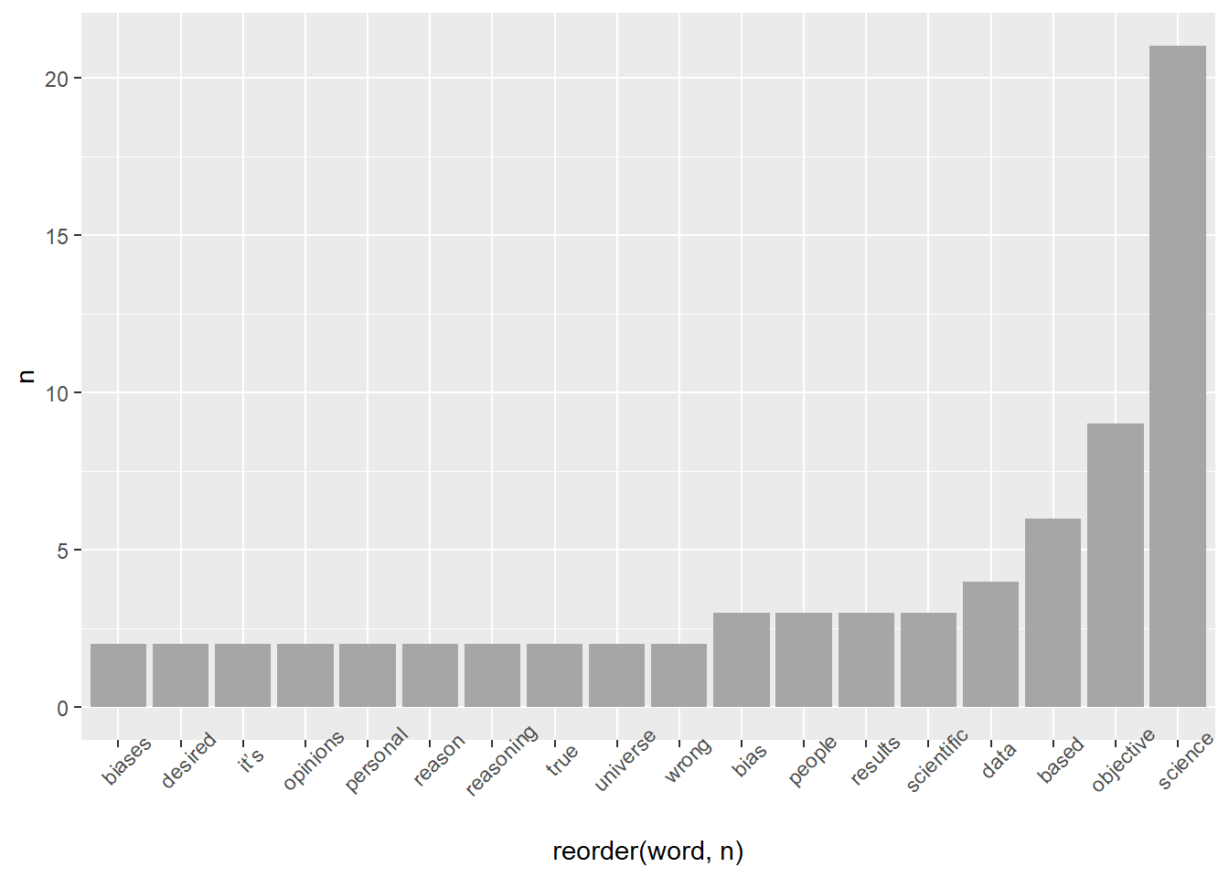
Now lets do the same for the “No” responses and compare:
no_why <- no %>%
  select(`Why or why not?`) %>%
  unnest_tokens(output = word, #the new column name to put the text in
                input = `Why or why not?`)  %>%
  anti_join(stop_words, by = "word")
Snapshot of the word summary:
no_why %>%
  count(word, sort = TRUE)
## # A tibble: 211 × 2
## word n
## <chr> <int>
## 1 science 21
## 2 objective 15
## 3 research 11
## 4 subjective 10
## 5 results 8
## 6 data 6
## 7 bias 5
## 8 biases 5
## 9 humans 5
## 10 objectivity 5
## # … with 201 more rows
## # ℹ Use `print(n = ...)` to see more rowsno_why %>%
count(word) %>%
filter(n >1) %>%
ggplot(aes(x = reorder(word,n), y = n))+ #reorder makes the bars go in order high to low
geom_col()+
scale_y_continuous(expand = c(0,0))+
theme(axis.text.x = element_text(angle = 45))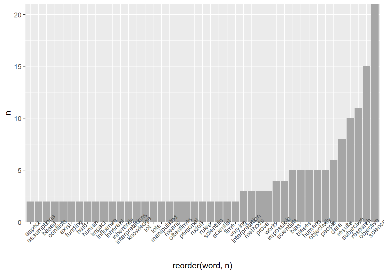
Let’s compare the top 5 words in “Yes” vs. “No” by binding our dataframes and faceting:
yes_summary <- yes_why %>%
  count(word) %>%
  # take the top 5
  top_n(5) %>%
  # create a new variable we can facet by later
  mutate(answer = "Yes")


# do the same for No
no_summary <- no_why %>%
  count(word) %>%
  # take the top 5
  top_n(5) %>%
  # create a new variable we can facet by later
  mutate(answer = "No")
Now bind these into one data frame and compare the answers
bind_rows(yes_summary, no_summary) %>%
  ggplot(aes(x = reorder(word,n), y = n))+
  geom_col()+
  facet_wrap(~answer)+
  theme(axis.text.x = element_text(angle = 45))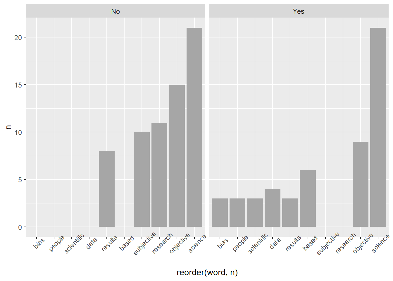
Another way to compare the answers is to calculate the proportion of each word in the dataset and create a correlation plot
bind_rows(mutate(yes_why, answer = "yes"),
          mutate(no_why, answer = "no"))%>%
  group_by(answer) %>%
  count(word) %>%
  mutate(proportion = n / sum(n)) %>%
  select(-n) %>%
  pivot_wider(names_from = answer, values_from = proportion) %>%
  ggplot(aes(x = no, y = yes))+
  geom_jitter(color = "black")+
  geom_text(aes(label = word), color = "black", check_overlap = TRUE, vjust = 1)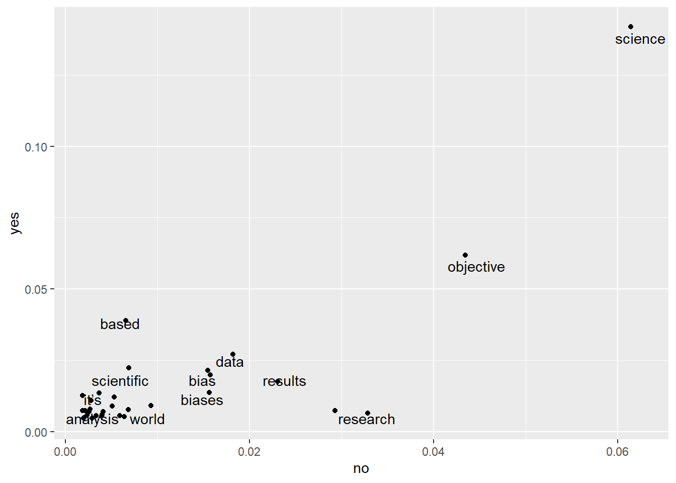
10.0.2 What are the pros and cons of open science?
Next, let’s analyze the responses describing the pros and cons to open science.
For this example let’s compare the responses using n-grams, which looks at adjacent words instead of just single words, so we can detect common phrases and word associations. The process is similar as before, using the unnest_tokens() function, but this time we add the argument token = "ngrams". We also specify n for how many consecutive words to examine, starting with an n = 2 argument which is often called a ‘bigram’.
Let’s start analyzing the pros of open science:
pros_bigrams <- data %>%
  select(ID, text = `What do you think are the pros of open science?`) %>%
  unnest_tokens(bigram, text, token = "ngrams", n = 2)
Examine the most common pairs of words:
pros_bigrams %>%
  count(bigram, sort = TRUE)
## # A tibble: 709 × 2
## bigram n
## <chr> <int>
## 1 open science 18
## 2 of open 8
## 3 access to 7
## 4 can be 7
## 5 pros of 7
## 6 able to 6
## 7 allows for 6
## 8 i think 5
## 9 more people 5
## 10 are able 4
## # … with 699 more rows
## # ℹ Use `print(n = ...)` to see more rowsLet’s clean this us by removing stop words. Since we now have a column with two word strings instead of one, we have to clean this a little differently. First, we use separate() to convert our single column into two, and specify that the empty space is our separator. Then we filter out stop words from both columns.
pros_bigrams %>%
  separate(bigram, into = c("word1", "word2"), sep = " ") %>%
  filter(!word1 %in% stop_words$word) %>%
  filter(!word2 %in% stop_words$word) %>%
  count(word1, word2, sort = TRUE)
## # A tibble: 92 × 3
## word1 word2 n
## <chr> <chr> <int>
## 1 community collaboration 2
## 2 makes science 2
## 3 saves time 2
## 4 science community 2
## 5 science makes 2
## 6 share knowledge 2
## 7 access articles 1
## 8 access information 1
## 9 access knowledge 1
## 10 allowing people 1
## # … with 82 more rows
## # ℹ Use `print(n = ...)` to see more rowsNow we can see the most common pairs of words in the responses that don’t contain noise/stop words. Lets do the same for the cons of open science:
cons_biograms <- data %>%
  select(ID, text = `What do you think are the cons of open science?`) %>%
  unnest_tokens(bigram, text, token = "ngrams", n = 2)
Now clean and summarize:
cons_biograms %>%
  separate(bigram, into = c("word1", "word2"), sep = " ") %>%
  filter(!word1 %in% stop_words$word) %>%
  filter(!word2 %in% stop_words$word) %>%
  count(word1, word2, sort = TRUE)
## # A tibble: 89 × 3
## word1 word2 n
## <chr> <chr> <int>
## 1 sensitive information 3
## 2 data privacy 2
## 3 false data 2
## 4 intellectual property 2
## 5 sensitive data 2
## 6 access articles 1
## 7 access fees 1
## 8 acquired data 1
## 9 actual researchers 1
## 10 applicable due 1
## # … with 79 more rows
## # ℹ Use `print(n = ...)` to see more rows10.0.3 Contribute to Equity and Environmental Justice
Lastly, let’s work with the survey question ‘In what ways do you believe you can contribute to equity and environmental justice?’
Let’s first analyze the most common words in the data set, and make a word cloud using the wordcloud package.
data %>%
  select(`In what ways do you believe you (in any aspect of your life or career) can contribute to equity and environmental justice?`) %>%
  unnest_tokens(output = word, #the new column name to put the text in
                input = `In what ways do you believe you (in any aspect of your life or career) can contribute to equity and environmental justice?`)  %>%
  anti_join(stop_words, by = "word") %>%
  count(word) %>%
  # make the wordcloud
  with(wordcloud(
    words = word,
    freq = n,
    random.order = FALSE,
    scale = c(2, 0.5),
    min.freq = 2,
    max.words = 100,
    colors = c("#6FA8F5",
               "#FF4D45",
               "#FFC85E")
  ))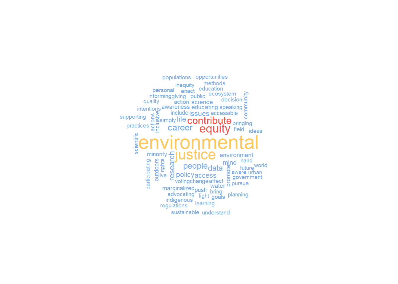
Looks like the most common words are pretty repetitive of those in the original question. Lets look at the ngrams for these responses, and try looking at phrases by pulling three consecutive words at a time.
data %>%
  select(ID, text = `In what ways do you believe you (in any aspect of your life or career) can contribute to equity and environmental justice?`) %>%
  unnest_tokens(bigram, text, token = "ngrams", n = 3) %>%
  separate(bigram, into = c("word1", "word2", "word3"), sep = " ") %>%
  filter(!word1 %in% stop_words$word) %>%
  filter(!word2 %in% stop_words$word) %>%
  filter(!word3 %in% stop_words$word) %>%
  count(word1, word2, word3, sort = TRUE)
## # A tibble: 41 × 4
## word1 word2 word3 n
## <chr> <chr> <chr> <int>
## 1 environmental justice issues 4
## 2 activism giving donations 1
## 3 address environmental injustices 1
## 4 addressing environmental justice 1
## 5 change policy implementations 1
## 6 collecting environmental data 1
## 7 conducting research related 1
## 8 disproportionately affect minority 1
## 9 donations volunteering conducting 1
## 10 ecosystem management planning 1
## # … with 31 more rows
## # ℹ Use `print(n = ...)` to see more rows