3 Introduction to R and RStudio
3.1 Getting to know RStudio
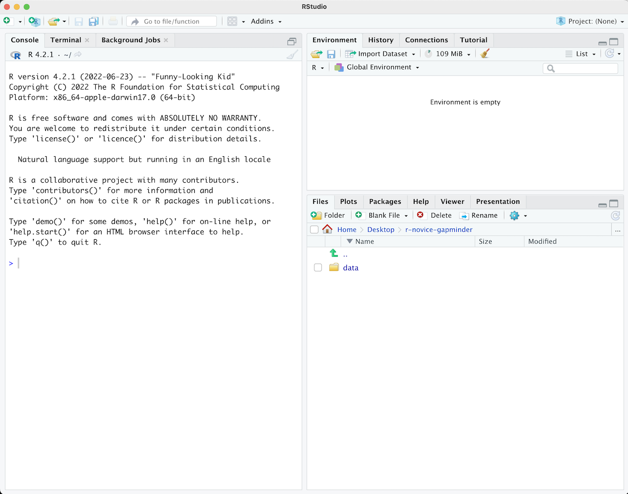
When you first open RStudio, it is split into 3 panels:
- The Console (left), where you can directly type and run code (by hitting Enter)
- The Environment/History pane (upper-right), where you can view the objects you currently have stored in your environment and a history of the code you’ve run
- The Files/Plots/Packages/Help pane (lower-right), where you can search for files, view and save your plots, view and manage what packages are loaded in your library and session, and get R help

Image Credit: Software Carpentry
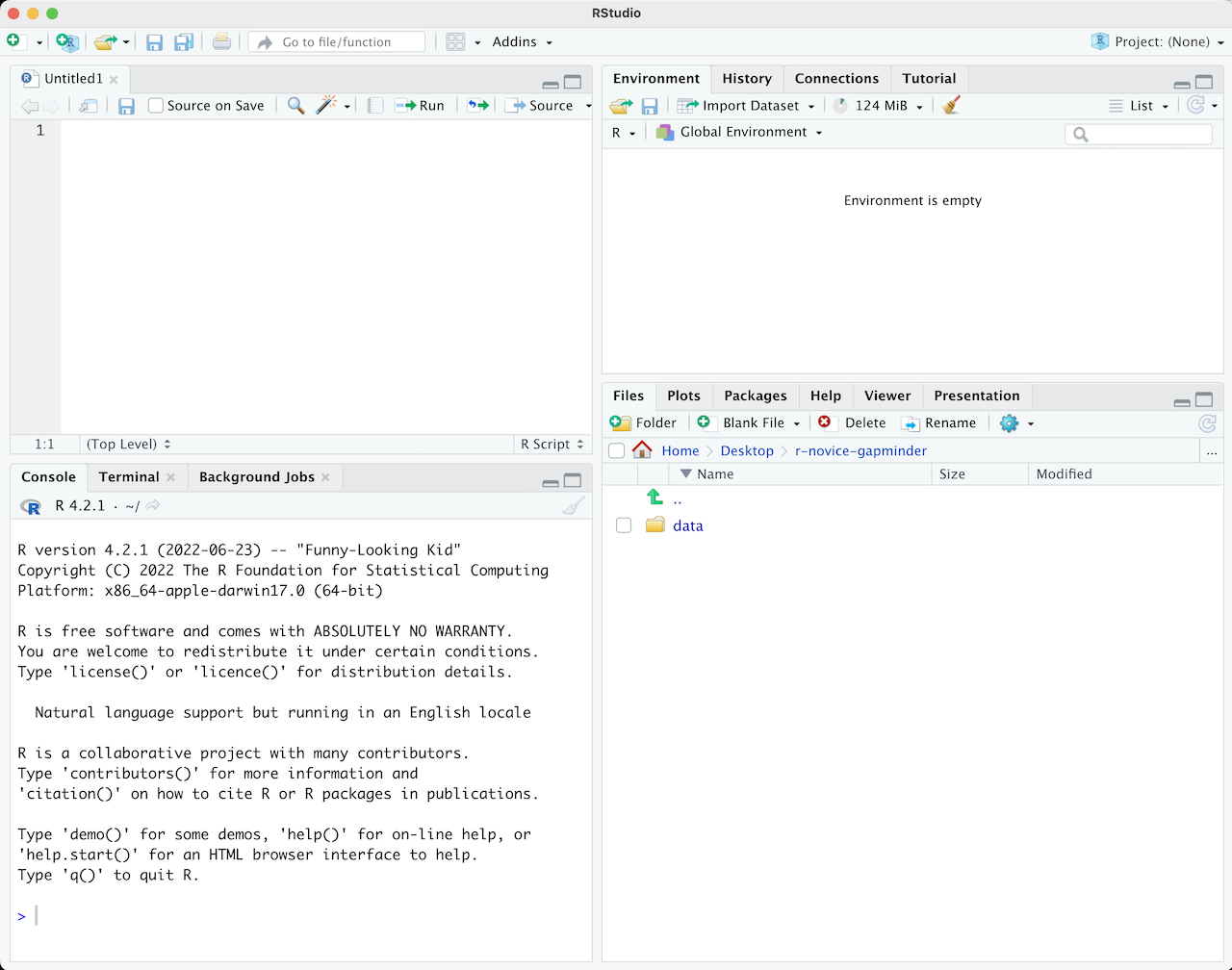
To write and save code you use scripts. You can open a new script with File -> New File -> R Script or by clicking the icon with the green plus sign in the upper left corner under ‘File’. When you open a script, RStudio then opens a fourth ‘Source’ panel in the upper-left to write and save your code. You can also send code from a script directly to the console to execute it by highlighting the entire code line/chunk (or place your cursor at the very end of the code chunk) and hit CTRL+ENTER on a PC or CMD+ENTER on a Mac.

Image Credit: Software Carpentry
It is good practice to add comments/notes throughout your scripts to document what the code is doing. To do this start your text with a #. R knows to ignore everything after a #, so you can write whatever you want there. Note that R reads line by line, so if you want your comments to carry over multiple lines you need a # at every line.
3.2 R Projects
As a first step whenever you start a new project, workflow, analysis, etc., it is good practice to set up an R project. R Projects are RStudio’s way of bundling together all your files for a specific project, such as data, scripts, results, figures. Your project directory also becomes your working directory, so everything is self-contained and easily portable.
We recommend using a single R Project for this course, so lets create one now.
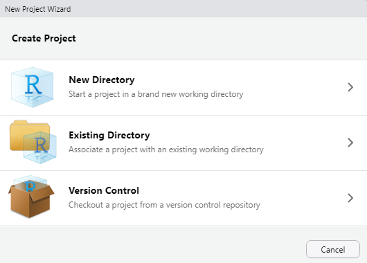
You can start an R project in an existing directory or in a new one. To create a project go to File -> New Project:

Let’s choose ‘New Directory’ then ‘New Project’. Now choose a directory name, this will be both the folder name and the project name, so use proper spelling conventions (no spaces!). We recommend naming it something course specific, like ‘ESS-330-2023’. Choose where on your local file system you want to save this new folder/project, then click ‘Create Project’.
Now you can see your RStudio session is working in the R project you just created. You can see the working directory printed at the top of your console is now the project directory, and in the ‘Files’ tab in RStudio you can see there is an .Rproj file with the same name as the R project, which will open up this R project in RStudio whenever you come back to it.
Test out how this .Rproj file works. Close out of your R session, navigate to the project folder on your computer, and double-click the .Rproj file.
What is a working directory? A working directory is the default file path to a specific file location on your computer to read files from or save files to. Since everyone’s computer is unique, everyone’s full file paths will be different. This is an advantage of working in R Projects, you can use relative file paths, since the working directory defaults to wherever the .RProj file is saved on your computer you don’t need to specify the full unique path to read and write files within the project directory.
3.3 Write your first script
Let’s start coding!
The first thing you do in a fresh R session and at the beginning of a workfow is set up your environment, which mostly includes installing and loading necessary libraries and reading in required data sets. Let’s open a fresh R script and save it in our root (project) directory. Call this script something like ‘r-intro.R’.
3.3.1 Commenting code
It is best practice to add comments throughout your code noting what you are doing at each step. This is helpful for both future you (say you forgot what a chunk of code is doing after returning to it months later) and for others you may share your code with.
To comment out code you use a #. You can use as many #’s as you want, any thing you write on that line after at least one # will be read as a comment and R will know to ignore that and not try to execute it as code.
At the top of your script, write some details about the script like a title, your name and date.
# Introduction to R and RStudio
# your name
# date
Now for the rest of this lesson, write all the code in this script you just created. You can execute code from a script (i.e., send it from the script to the console) in various ways (see below). Think of these scripts as your code notes, you can write and execute code, add notes throughout, and then save it and come back to it whenever you want.
3.3.2 Executing code
Almost always you will start a script by installing and/or loading all the libraries/packages you need for that workflow. Add the following lines of code to your script to import our R packages you should have already installed from the R Setup page.
#load necessary libraries
library(tidyverse)
library(palmerpenguins)
To execute code you can either highlight the entire line(s) of code you want to run and click the ‘Run’ button in the upper-right of the Source pane or use the keyboard shortcut CTRL+Enter on Windows or CMD+Enter on Macs.
You can also place your cursor at the very end of the line or chunk of code you want to run and hit CTRL+Enter or CMD+Enter.
All functions and other code chunks must properly close all parentheses or brackets to execute. If you have an un-closed parentheses/bracket you will get stuck in a never ending loop and will keep seeing + printed in the console. To get out of this loop you can either close the parentheses or bracket, or hit ESC to start over. You want to make sure you see the > in the console and not the + to execute code.
3.3.3 Getting help with code
Take advantage of the ‘Help’ pane in RStudio! There you can search packages and specific functions to see all the available and required arguments, along with the default argument settings and some code examples. You can also execute a help search from the console with a ?. For example:
?mean3.3.4 Functions
R has many built in functions to perform various tasks. To run these functions you type the function name followed by parentheses. Within the parentheses you put in your specific arguments needed to run the function.
Practice running these various functions and see what output is printed in the console.
# mathematical functions with numbers
log(10)

# average a range of numbers
mean(1:5)

# nested functions for a string of numbers, using the concatenate function 'c'
mean(c(1,2,3,4,5))


# functions with characters
print("Hello World")

paste("Hello", "World", sep = "-")
3.3.4.1 Assignment operator
Notice that when you ran the following functions above, the answers were printed to the console, but were not saved anywhere (i.e., you don’t see them stored as variables in your environment). To save the output of some operation to your environment you use the assignment operator <-. For example, run the following line of code:
x <- log(10)And now you see the output, ‘2.3025…’ saved as a variable named ‘x’. You can now use this value in other functions
x + 53.3.4.2 Base R vs. The Tidyverse
You may hear the terms ‘Base R’ and ‘Tidyverse’ a lot throughout this course. Base R includes functions that are installed with the R software and do not require the installation of additional packages to use them. The Tidyverse is a collection of R packages designed for data manipulation, exploration, and visualization that you are likely to use in every day data analysis, and all use the same design philosophy, grammar, and data structures. When you install the Tidyverse, it installs all of these packages, and you can then load all of them in your R session with library(tidyverse). Base R and Tidyverse have many similar functions, but many prefer the style, efficiency and functionality of the Tidyverse packages, and we will mostly be sticking to Tidyverse functions for this course.
3.3.5 Data Types
For this intro lesson, we are going to use the Palmer Penguins data set (which is loaded with the palmerpenguins package you installed during setup). This data was collected and made available by Dr. Kristen Gorman and the Palmer Station, Antarctica LTER, a member of the Long Term Ecological Research Network.
Load the penguins data set.
data("penguins")You now see it in the Environment pane. Print it to the console to see a snapshot of the data:
penguinsThis data is structured is a data frame, probably the most common data type and one you are most familiar with. These are like the spreadsheets you worked with in the first lesson, tabular data organized by rows and columns. However we see at the top this is called a tibble which is just a fancy kind of data frame specific to the tidyvese.
At the top we can see the data type of each column. There are five main data types:
character:
"a","swc"numeric:
2,15.5integer:
2L(theLtells R to store this as an integer, otherwise integers can also be numeric data types)logical:
TRUE,FALSEcomplex:
1+4i(complex numbers with real and imaginary parts)
Data types are combined to form data structures. R’s basic data structures include
atomic vector
list
matrix
data frame
factors
You can see the data type or structure of an object using the class() function, and get more specific details using the str() function. (Note that ‘tbl’ stands for tibble).
class(penguins)
str(penguins)class(penguins$species)
str(penguins$species)When we pull one column from a data frame, like we just did above with the $ operator, that returns a vector. Vectors are 1-dimensional, and must contain data of a single data type (i.e., you cannot have a vector of both numbers and characters).
If you want a 1-dimensional object that holds mixed data types and structures, that would be a list. You can put together pretty much anything in a list.
myList <- list("apple", 1993, FALSE, penguins)
str(myList)
You can even nest lists within lists
list(myList, list("more stuff here", list("and more")))You can use the names() function to retrieve or assign names to list and vector elements
names(myList) <- c("fruit", "year", "logic", "data")
names(myList)
3.3.6 Indexing
Indexing is an extremely important aspect to data exploration and manipulation. In fact you already started indexing when we looked at the data type of individual columns with penguins$species. How you index is dependent on the data structure.
Index lists:
# for lists we use double brackes [[]]
myList[[1]]

myList[["data"]]
Index vectors:
# for vectors we use single brackets []
myVector <- c("apple", "banana", "pear")
myVector[2]
Index data frames:
# dataframe[row(s), columns()]
penguins[1:5, 2]

penguins[1:5, "island"]

penguins[1, 1:5]

penguins[1:5, c("species","sex")]

penguins[penguins$sex=='female',]

# $ for a single column
penguins$species
3.3.7 Read and Write Data
We used an R data package today to read in our data frame, but that probably isn’t how you will normally read in your data. There are many ways to read and write data in R. To read in .csv files, you can use read_csv() which is included in the Tidyverse with the readr package, and to save csv files use write_csv(). The readxl package is great for reading in excel files, however it is not included in the Tidyverse and will need to be loaded separately.
Find the .csv you created at the end of last week’s lesson. Created a folder in your project directory called ‘data/’ and copy the .csv file there. You will store various data sets in this ‘data/’ folder throughout the course.
Say your .csv is called ‘survey_data_clean.csv’. This is how you would read it in to R, giving it the object name ‘survey_data’
survey_data <- read_csv("data/survey_data_clean.csv")3.4 Exercises
For each question you must also include the line(s) of code you used to arrive at the answer.
Use
class()andstr()to inspect the .csv you created from last week’s lesson that you just read into R. How many rows and columns does it have? What data type is each column? (4 pts)Why don’t the following lines of code work? Tweak each one so the code runs (6 pts)
myList[year]penguins$flipper_lenght_mmpenguins[island=='Dream',]How many species are in the
penguinsdataset? What islands were the data collected for? (Note: theunique()function might help) (5 pts)Use indexing to create a new data frame that has only 3 columns: species, island and flipper length columns, and subset all rows for just the ‘Dream’ island. (5 pts)
Use indexing and the
mean()function to find the average flipper length for the Adelie species on Dream island. (5 pts)